Kosaraju 学习笔记
Fountaine_of_Belleau
·
·
个人记录
\texttt{Chapter zero: Kosaraju 的来历}
(以上内容来自 [oi-wiki](https://oi-wiki.org/graph/scc/))
### $\texttt{Chapter one: 何为强连通分量}
强连通分量的定义是:极大的强连通子图。
一个更加通俗的定义是:一个有向图中的极大子集,使得其中任意两个点都互相连通。特别地,一个点也是强连通分量。
如图所示:
为了方便表示,下文中的 \texttt{SCC(Strongly Connected Components)} 表示强连通分量。
\texttt{Chapter two: 算法过程}
第一遍 $\texttt{Dfs}$ 先在原图中求出每个点的时间戳,并将其压入栈中:
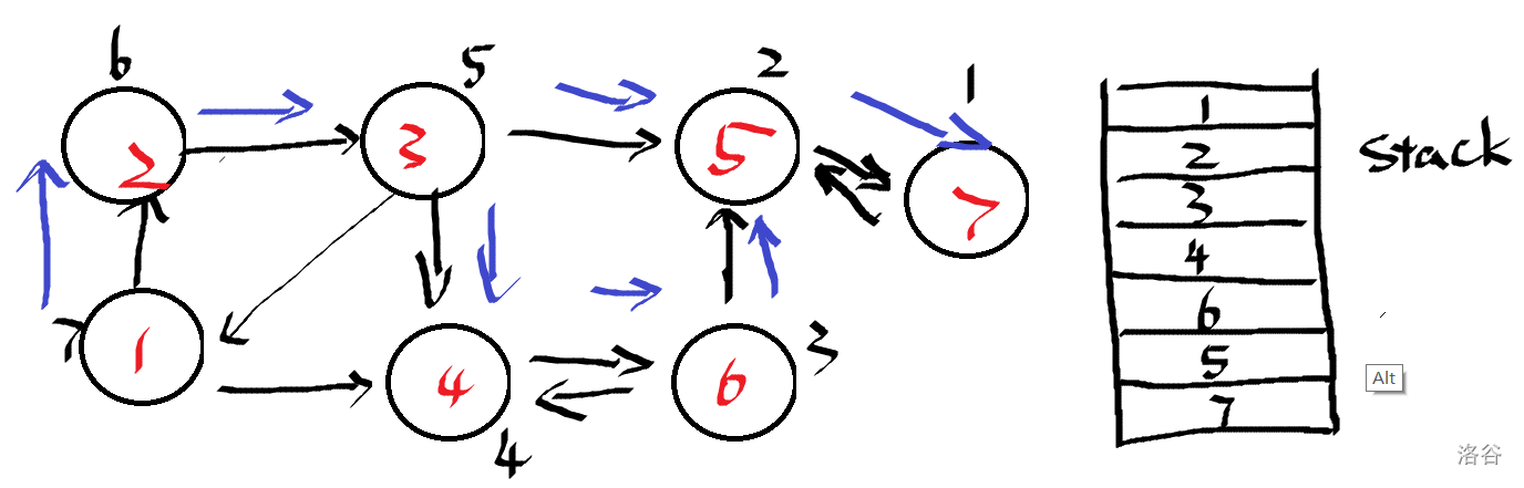
第二遍 $\texttt{Dfs}$ 则要从栈顶开始遍历反图,并求出 $\texttt{SCC}$。
为了证明 $\texttt{Kosaraju}$ 算法的正确性,我们需要证明原图和反图的连通性相同。
证明:我们可以将有向图具象化为两个点:$\texttt{V1, V2}$。
如果在原图中 $\texttt{V1}$ 有一条路径到达 $\texttt{V2}$,则有一条链:$\texttt{V1} \to \texttt{V2}$,如果将其反转,则有一条链 $\texttt{V2} \to \texttt{V1}$。
所以,我们可以推出如果 $\texttt{V1} \to \texttt{V2}$ 与 $\texttt{V2} \to \texttt{V1}$ 同时存在,则将其反转时连通性不变。其他情况,则连通性必然改变。
如此,算法的正确性得证。
时间复杂度:显然,每遍 $\texttt{Dfs}$ 都会经过每个点、每条边恰好一次,所以时间复杂度为 $\Theta(V + E)$。
下面是参考代码:
```cpp
void Dfs1(int cur) {
_vis[cur] = 1;
for (int i = 0; i < _gr[cur].size(); i++) {
if (!_vis[_gr[cur][i]]) {
Dfs1(_gr[cur][i]);
}
}
_st.push_back(cur);
}
void Dfs2(int cur) {
_col[cur] = _tot;
for (int i = 0; i < _rev[cur].size(); i++) {
if (!_col[_rev[cur][i]]) {
Dfs2(_rev[cur][i]);
}
}
}
void Kosaraju() {
for (int i = 1; i < _node + 1; i++) {
if (!_vis[i]) {
Dfs1(i);
}
}
for (int i = _node - 1; i > -1; i--) {
if (!_col[_st[i]]) {
_tot++;
Dfs2(_st[i]);
}
}
}
```
### $\texttt{Chapter three: 例题、应用}
- P2863 [USACO06JAN]The Cow Prom S 强连通分量板子题
- 2341 [USACO03FALL][HAOI2006]受欢迎的牛 G 稍微难一点的应用
- P3387 【模板】缩点 强连通分量+缩点
- P1073 [NOIP2009 提高组] 最优贸易 强连通分量+缩点+dp
参考代码